Plot a trait: distribution and field map

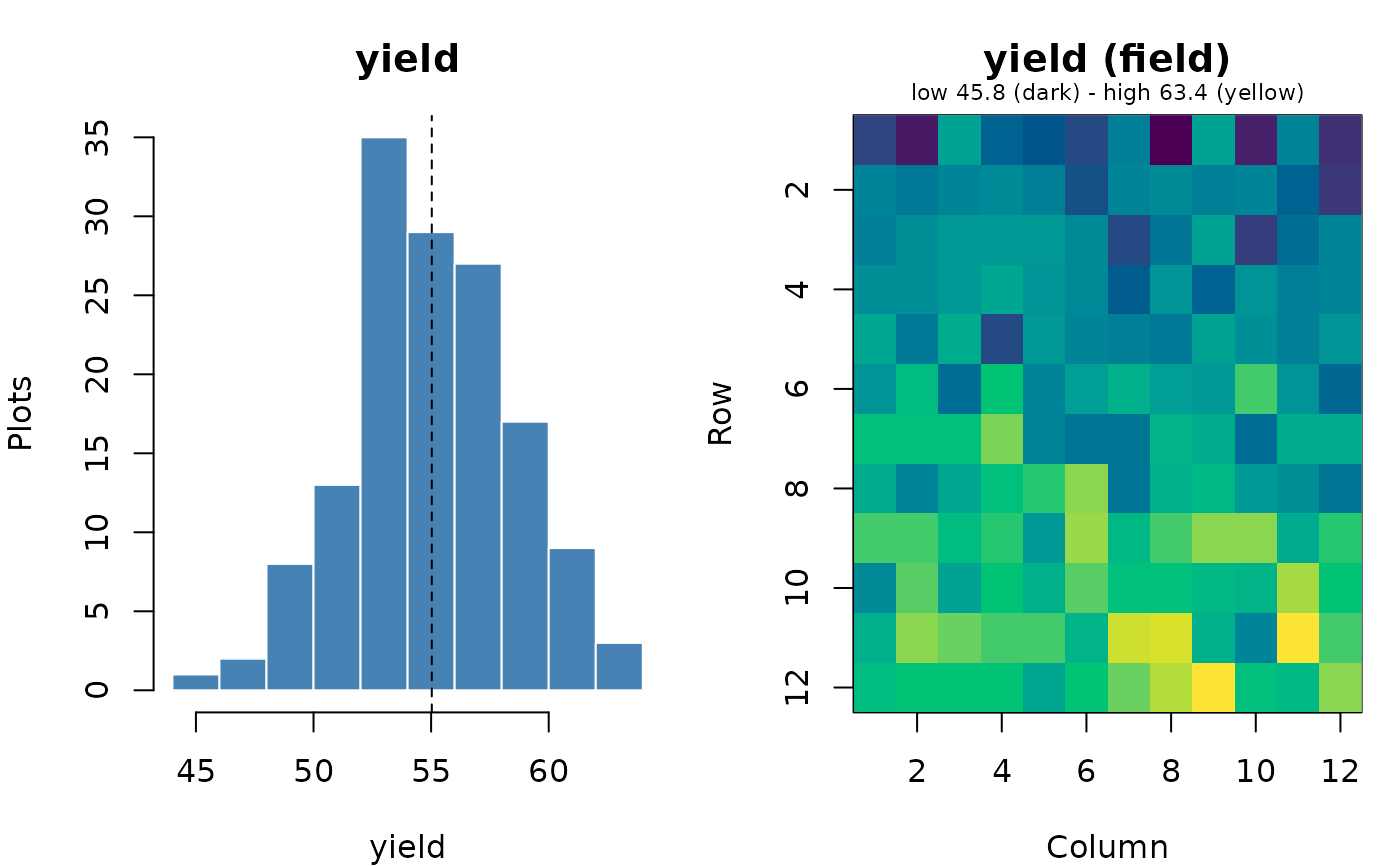
Draws, for each location (or other group), a histogram of the trait and a map of the field with the value of every plot, so gradients, odd plots and outliers are easy to see. Outliers from find_outliers() can be circled on the map.

Usage

plot_trait(
  data,
  trait,
  by = if ("location" %in% names(data)) "location" else NULL,
  type = c("both", "histogram", "field"),
  row_col = "row",
  col_col = "col",
  outliers = NULL,
  breaks = "Sturges"
)

Arguments

data

A data frame with one row per plot.

trait

Name of the numeric trait column.

by

Optional grouping column; by default "location" when the data have it.

type

"both" (histogram and field map), "histogram" or "field".

row_col, col_col

Field row and column columns (for the map).

outliers

Optional table from find_outliers() to circle on the map.

breaks

Histogram breaks, as in graphics::hist().

Value

Invisibly, a tibble with a summary per group: plots, values, missing, mean, sd, min, max and CV (%).

Examples

rc <- augmented_row_column_design(paste0("G", 1:108), paste0("C", 1:4),
                                  12, 12, 4, 4, n_candidates = 5, seed = 1)
d <- rc$design
d$yield <- 50 + 0.8 * d$row + rnorm(nrow(d), sd = 2)
plot_trait(d, "yield")