Compare raw and first-stage adjusted values

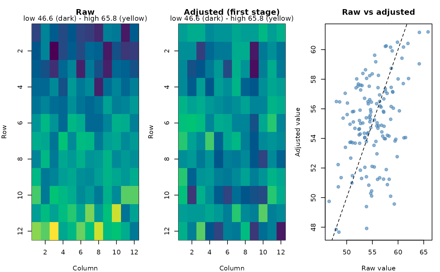
Puts each plot's raw value next to its first-stage value (the genotype's adjusted mean plus the plot's residual, as in first_stage_values()), summarises how much the first stage changed (per location: correlation of raw and adjusted plot values, the spread before and after, and how much the ranking of the genotypes changed) and draws, per location, the raw and the adjusted field maps and a raw-versus-adjusted plot.

Usage

compare_first_stage(fit, plot = TRUE, locations = NULL)

Arguments

fit

An analysis (e.g. analyze_augmented_row_column_design() with spatial = TRUE) or a two-stage analysis (analyze_two_stage(), analyze_augmented_prep_two_stage()), whose stage-1 fits are compared.

plot

Logical. Draw the plots.

locations

For two-stage analyses: the locations to draw (default all).

Value

Invisibly, a list with plots (one row per plot: location, plot, genotype, row, col, raw, adjusted, change) and summary (one row per location). The summary is also printed.

Examples

rc <- augmented_row_column_design(paste0("G", 1:108), paste0("C", 1:4),
                                  12, 12, 4, 4, n_candidates = 5, seed = 1)
d <- rc$design
set.seed(1)
d$yield <- 50 + 0.8 * d$row + rnorm(nrow(d), sd = 2)
fit <- analyze_augmented_row_column_design(d, "yield")
cmp <- compare_first_stage(fit)
#> Raw versus first-stage adjusted values:
#>  location plots cor_raw_adjusted sd_raw sd_adjusted genotype_rank_cor
#>     trial   144            0.384    3.6        2.89             0.314
#>  top10pct_kept
#>            0.5
#> (genotype_rank_cor: Spearman correlation of genotype means; top10pct_kept: share of the raw top 10% still in the adjusted top 10%)